Lec 5 GPUs

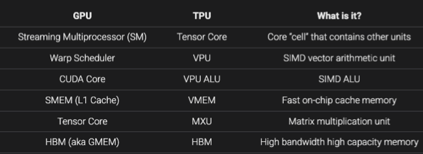
GPU 结构

硬件层:

• GPU
• 1 GPU = 多个 SM (streaming multiprocessor)
• 1 SM = 4 warp schedulers
• 1 SM = 多个 SP (streaming processor)

应用层（被动态分配到硬件层）:

• 1 cuda app
• 1 app =4096 blocks (每个动态分配到一个 SM)
  • 1 block 有自己的 shared memory
  • 1 block = 8 warps
  • 1 warp = 32 threads
  • 1 thread 有自己的 register
• 多个 blocks in 1 grid （这 grid 是硬件吗）
  • 1 grid 有自己的 global memory(CPU DRAM) 和 constant memory

优化技巧 1: 低精度运算

• 前沿 : MXFP8
• 关于量化:
• 所有权重包括FFN 和 QKV 矩阵都支持 fp32 到 fp8 量化吗？
  • [gemini] yes。但部分最终层 head 可能保留
• 大概多少数据共享一个 scailing factor? 相邻数据的数量级在实际模型中会比较接近吗（否则就没法相邻数据用 scailing factor吧）？
  • [gemini] (1x32) 或者 (32x1)
  • 在模型训练或存储时，编译器会进行重排，尽量让数值相关性强的权重放在同一个 Tile（块）里

优化技巧 2: Operator fusion 算子融合

• Computing sin2𝑥 + cos2 𝑥 naively launches 5 CUDA kernels (back and forth)
• ‘Easy’ fusions like this can be done automatically by compilers (torch.compile)

优化技巧3: recomputing 不要缓存

三个连续的 sigmoid，forward 进行 3 次 write（存梯度），backward 进行 3 次 read(取梯度)，浪费带宽。不如直接不存梯度，反向传播的时候从 x 开始重新直接算梯度

优化技巧4 : Memory coalescing with DRAM

• ? For row-major matrices – threads that move along rows are not coalesced. Note how the second diagram reads the entire vector at each step!

Trick 5 (the big one): tiling 矩阵分块

一种提升缓存效率的方法.

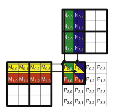
Matrix mystery

Part 1: tiling: 矩阵形状最好是 2^n，比如64比4更好

Part 2: wave quantization: 矩阵从1792x1792到 1793x1793, tile 数量增加到刚好超出A100的SM数量，导致A100无法同时执行所有的 tiles.

Flash attn

• Tiling part 1: tiling for the KQV matrix multiply
• Tiling part 2: incremental computation of the softmax (telescoping sum trick)

SM 的 shm 和 L1 的区别：shm 由程序员手动控制，而 L1 不可见.

Lec6 Tritons:

上节课补充:

• All threads within a warp must execute same instructions in lockstep on an SM. if different threads in a warp need to execute different instructions (if A, else B), must be done sequentially (bad)
• SM 的 warp 调度器支持异步（例如一个 warp 被 IO 阻塞了）
• SM occupancy 指的是 实际调度的 warp 数（随着可变的 num_registers_per_thread 变化，受限于出厂固定的 num_threads_per_block 和 max_registers_per_sm） / SM 支持的 warp 调度器数量. 这个 occupancy 低不一定坏

Lec9 S C A L I N G L A W S

• skip most of this part

HW3 4 5

• 3. 简单 scailing law
• 4. 数据清洗
• 5. PPO/RL (GRPO)

Lec 10: Inference

• 标准 grouped query transformer 字母图: https://cs336.stanford.edu/lectures?trace=lecture_10&step=47

[gemini]

1. 推理与训练的特性截然不同：训练（Prefill 阶段）可以并行计算，通常是计算密集型（Compute-bound）；而推理的生成阶段（Generation 阶段）是自回归的，通常是内存带宽密集型（Memory-bound）。
2. 算术强度（Arithmetic Intensity）决定瓶颈：算术强度（FLOPs / Bytes）如果小于硬件的加速器强度，系统就是内存受限的。在生成阶段，算术强度极低，因为每次只生成一个 token 就需要加载庞大的模型参数和 KV Cache。
3. Batching（批处理）的作用与局限：在 MLP 层，增大 Batch Size 可以有效提高算术强度，缓解内存带宽瓶颈；但在 Attention 层，每个序列都有独立的 KV Cache，增大 Batch Size 无法提高 Attention 层的算术强度（始终小于 1）。
4. 减小 KV Cache 是核心优化方向：由于生成阶段受限于内存，减少 KV Cache 的大小（不显著损失精度）是提高吞吐量和降低延迟的关键。
5. GQA（分组查询注意力）：通过让多个 Query 头共享少量的 Key/Value 头，大幅减少 KV Cache 的大小，同时保持接近 MHA（多头注意力）的生成质量。
6. MLA（多头潜在注意力）：DeepSeek 提出的架构，将 KV Cache 压缩为一个低维的潜在向量（Latent Vector），在需要时再投影恢复，从而极大地减少了 KV Cache 的内存占用（如 DeepSeek-V2 减少了 93.3%）。
7. CLA（跨层注意力）：在 GQA 的基础上进一步优化，让相邻的层（Layers）也共享 Key 和 Value 头，可以再将 KV Cache 缩小 2 倍。
8. 量化（Quantization）：通过降低数值精度（如使用 AWQ 等激活感知量化技术），减少内存占用和数据传输量，从而直接提升内存受限下的推理速度。
9. 投机采样（Speculative Sampling/Decoding）：利用“验证比生成快”的非对称性，使用一个小模型（Draft Model）快速生成多个候选 token，再由大模型（Target Model）并行验证，从而在**不损失精度（Lossless）**的情况下加速推理。
10. 动态工作负载的系统级优化（如 vLLM 的 PagedAttention）：借用操作系统中虚拟内存和分页（Paging）的思想，解决动态序列长度导致的 KV Cache 内存碎片化问题，实现近乎零浪费的内存管理，大幅提升并发吞吐量。