Papers batch 1

RT-2 (1)

• https://hjfy.top/arxiv/2307.15818 和 OpenVLA 同属一派，将 VLM 的最后 256 个 token id 分配给动作，直接将 x, y, z, yaw, pitch, roll, gripper 划分为 256 个离散桶，七个动作维度共享 token id 并通过位置区分语义，直接拼接丢给 VLM 输出隐状态，一个 head 解码出 id 再映射回动作空间. 缺点是离散化和自回归导致的精度不够.

RT-1 输出的同样为离散词表，只不过是从零开始训练小型 transformer.

TODO: 数据集这一块儿有空可以再看看.

World Model for Robot Learning: A Comprehensive Survey (2)

• https://hjfy.top/arxiv/2605.00080

Fast-WAM (Yuanet al., 2026) (3)

• https://hjfy.top/arxiv/2603.16666

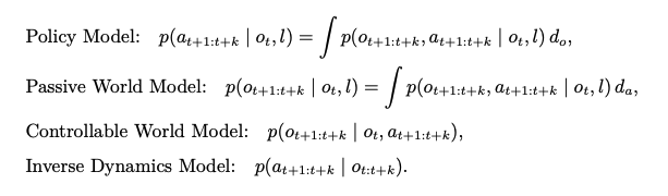
可被视为该家族中的一个混合点：它采用具有共享注意力的 Transformer 混合体骨干网络 及耦合的视频与动作分支，但结论认为主要优势可能更多来自训练期间的视频协同训练，而非推理阶段 的显式未来想象。在这些变体中，视频分支越来越不再被视为需要忠实渲染的输出，而是被看作一种预 测性潜在过程，其隐状态用于指导动作生成. (by 综述)

不论在 train-time 还是 infer-time, noisy action 都只会 attend 第一帧视频的 kv. infer-time 只需要把 clean obs_image 丢进 dit 前向跑一次生成 kv 给 action 用.

可以解释为，train-time 联合训练多帧视频和动作生成的好处是逼着 video z_0 编码能够“从当前画面推导出未来变化”的信息。Fast-wam 没有历史信息.

video loss: 让 z0 表征更懂未来/动力学

action loss: 让 action expert 学会从这个 z0 表征里采样动作

所谓双 DiT，其实就是 MoT，即 video DiT 和 action DiT 在每个 transformer layer 通过 self-attention 双向注意.

flowchart TD
    video["Training Video
(B, 3, T=33, H=224, W=448)"] --> vae["Wan VAE Encode"]
    vae --> z0["Video Latents z_0
(B, 48, T_lat=9, 28, 56)"]
    z0 --> zv["Add Flow Noise
sample t_v, eps_v"]
    zv --> vpre["Video Expert pre_dit
patchify + 3D RoPE"]

    prompt["Task Prompt / Cached Text
(B, L=128, D=4096)"] --> ctx["Text Context"]
    state["Robot State
(B, T, D_state=8)"] --> prop["proprio_encoder(Linear)
as 1 state token"]
    prop --> ctx
    ctx --> vpre

    action["GT Actions a_0
(B, T_act=32, A=7)"] --> za["Add Flow Noise
sample t_a, eps_a"]
    za --> apre["Action Expert pre_dit
Linear(A -> 1024) + 1D RoPE"]
    ctx --> apre

    vpre --> vt["Video Tokens
(B, S_v=3528, D_v=3072)"]
    apre --> at["Action Tokens
(B, 32, D_a=1024)"]
    vt --> mot["MoT Mixed Transformer
30 layers shared masked self-attn"]
    at --> mot
    mask["Mask
video->video causal
action->first-frame video + action"] --> mot

    mot --> vpost["Video post_dit
unpatchify"]
    mot --> apost["Action post_dit
Linear(1024 -> A)"]
    vpost --> pv["Predicted video velocity
(B, 48, T_lat', 28, 56)"]
    apost --> pa["Predicted action velocity
(B, 32, 7)"]

    zv --> vtgt["Target video velocity"]
    za --> atgt["Target action velocity"]
    pv --> vloss["Video FM Loss"]
    vtgt --> vloss
    pa --> aloss["Action FM Loss"]
    atgt --> aloss
    vloss --> total["Total Loss
lambda_v * L_video + lambda_a * L_action"]
    aloss --> total

Lingbot-va (4)

• https://hjfy.top/arxiv/2601.21998 Lin Li, Yinghao Xu

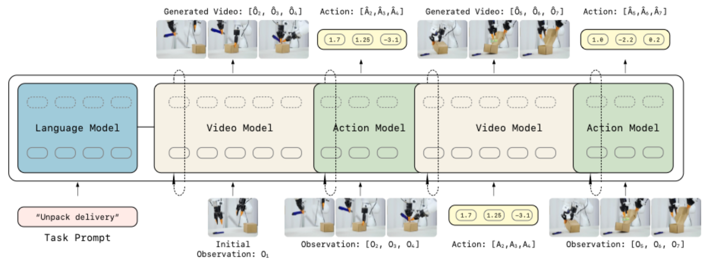
lingbot-va 的自回归扩散方法为：video/action diffusion 后对 clean token 计算 kv 存入 kv cache，此后 DiT 每一层将会 attend 之前的 kv. 而 diffusion 顺序为 video 2 帧 -> action 2x16 帧（这部分相当于 IDM） -> video 2 帧 -> action 2x16 帧，所有动作均会执行.

默认实现为 shared backbone，通过 action_mode 分支区分 video input 和 action input，它会选择不同的 input embedder, time embedder 和 output head. KV cache 使用 ring buffer 维护，容量约 9792 tokens.

1
obs0 -> VAE -> z0
2

3
infer #1 (frame_st_id=0):
4
1) flow denoise video chunk [z0_anchor, z1_hat]   # 2帧
5
   - 第0帧 init_latent=z0
6
   - 第1帧才是预测的未来 latent
7
2) flow denoise action chunk [a_grp0(16步), a_grp1(16步)]  # 1 action chunk = 2 group(对齐 2 video frame) = 32 steps
8
   - 条件：cache(空) + 刚预测的 video chunk
9

10
execute #1（第一轮特殊）:
11
    start_idx=1 -> 跳过 a_grp0，只执行 a_grp1 的 16 步
12
    每 4 步收一次 obs -> key_frame_list（约 4 个真实 obs）
13

14
compute_kv_cache #1:
15
    clear_pred_cache()          # 删掉 z_hat、a_hat，不是“替换某几帧”
18 collapsed lines
16
    real_z = VAE(key_frame_list)
17
    若 frame_st_id==0: cat(init_latent=z0, real_z)
18
    real_a = preprocess(executed action chunk)
19
    写入 cache（is_pred=False）
20

21
---
22

23
infer #2:
24
    预测下一个 chunk [z2_hat, z3_hat] + [a_grp2, a_grp3]
25
    条件：cache 里的 real history
26

27
execute #2 起:
28
    start_idx=0 -> 执行所有 32 步 action
29
    每 4 步收 obs -> key_frame_list（约 8 个）
30

31
compute_kv_cache #2:
32
    再次 clear_pred_cache()
33
    追加新的 real_z / real_a(real_a != pred_a)

Infer-time denoise video

flowchart TD
    cache["模块外 KV Cache
来自 compute_kv_cache #1
real history only: z/a KV
capacity per block: [B_eff=2, 9792, 24, 128]
这里 eff=2 是 CFG 用的"] -.-> attn
    noise_z["sample video noise
latents: [1, 48, 2, 24, 20]
表示 [z2_hat, z3_hat]"] --> prep["CFG repeat + grid/timestep
[B_eff=2, 48, 2, 24, 20]"]
    prep --> vemb[["patch_embedding_mlp
192 -> 3072"]]
    vemb --> vt["video tokens
seq_len = 2 * 12 * 10 = 240
[B_eff=2, 240, 3072]"]
    prompt["cached prompt_embeds
[B_eff=2, 512, 4096]"] --> textproj[["text_embedder
4096 -> 3072"]]
    textproj --> txt["text tokens
[B_eff=2, 512, 3072]"]
    vt --> attn[["Shared WanTransformerBlock x30
self-attn 读模块外 KV Cache
cross-attn 读 text tokens"]]
    txt --> attn
    attn --> vhead[["norm_out + proj_out"]]
    vhead --> vvel["video velocity
tokens [B_eff=2, 240, 192]
unpatch -> [B_eff=2, 48, 2, 24, 20]"]
    vvel --> sched["Flow scheduler step
更新 [z2_hat, z3_hat]"]
    sched --> predcache["最后一步 update_cache=1
把 predicted video KV 写入 cache
is_pred=True"]

Denoise action

flowchart TD
    cache["模块外 KV Cache
real history + 刚写入的 predicted video chunk KV
z/a history + [z2_hat,z3_hat]"] -.-> attn
    noise_a["sample action noise
actions: [1, 30, 2, 16, 1]
表示 [a_grp2, a_grp3]"] --> prep["CFG repeat + grid/timestep
[B_eff=2, 30, 2, 16, 1]"]
    prep --> aemb[["action_embedder
30 -> 3072"]]
    aemb --> at["action tokens
seq_len = 2 * 16 = 32
[B_eff=2, 32, 3072]"]
    prompt["cached prompt_embeds
[B_eff=2, 512, 4096]"] --> textproj[["text_embedder
4096 -> 3072"]]
    textproj --> txt["text tokens
[B_eff=2, 512, 3072]"]
    at --> attn[["Shared WanTransformerBlock x30
self-attn 读模块外 KV Cache
cross-attn 读 text tokens"]]
    txt --> attn
    attn --> ahead[["norm_out + action_proj_out"]]
    ahead --> avel["action velocity
[B_eff=2, 32, 30]
reshape -> [B_eff=2, 30, 2, 16, 1]"]
    avel --> sched["Flow scheduler step
更新 [a_grp2, a_grp3]"]
    sched --> predcache["最后一步 update_cache=1
把 predicted action KV 写入 cache
is_pred=True"]

RTC (5)

• https://arxiv.org/abs/2506.07339 | Kevin Black, Sergey

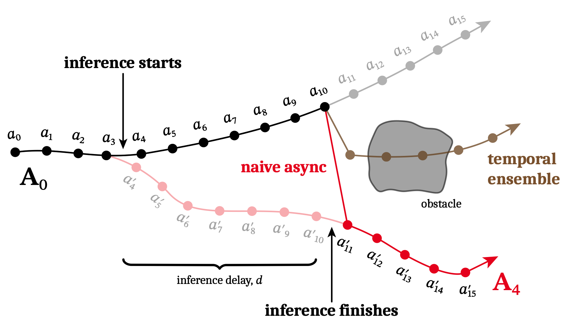
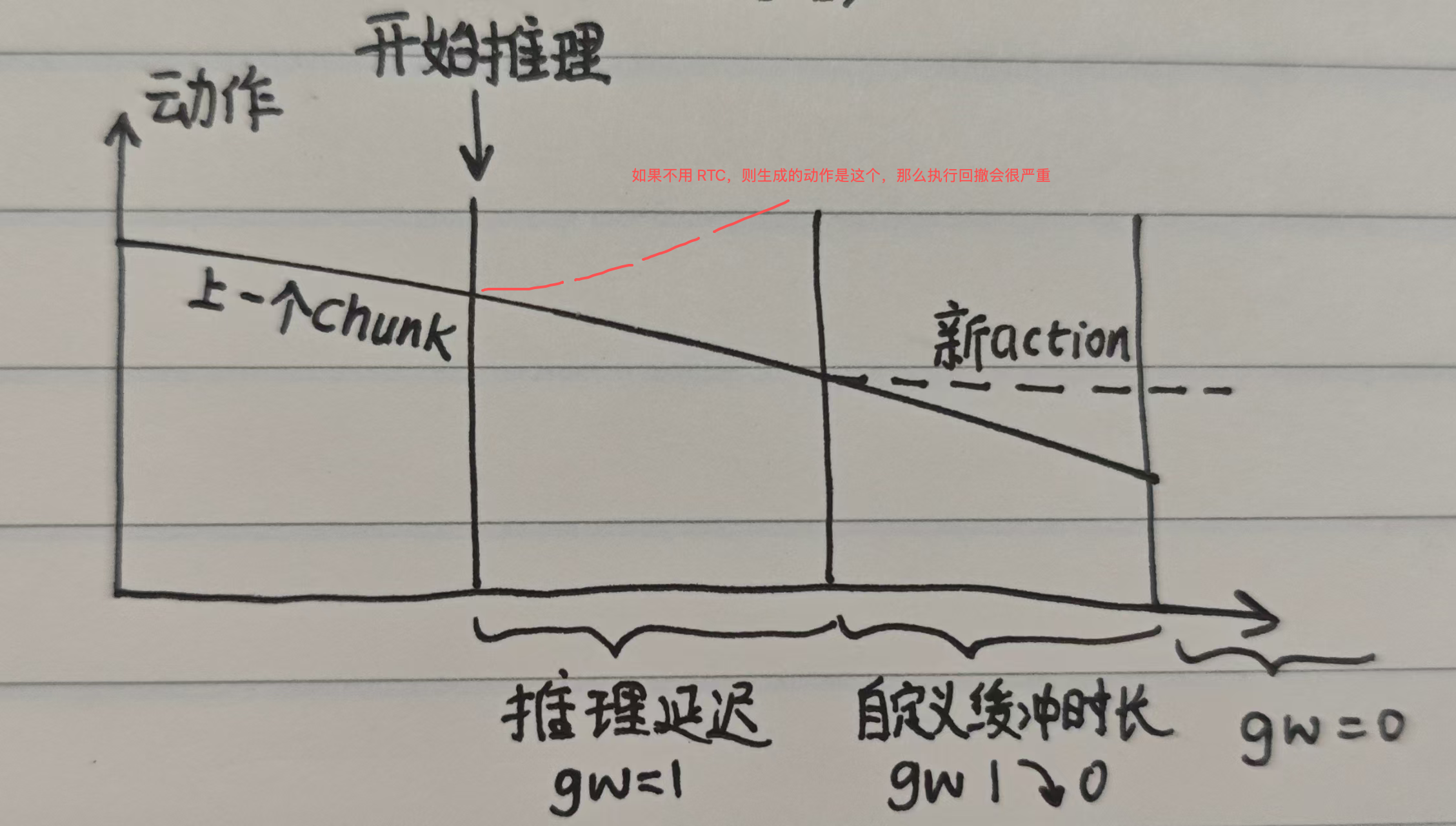
考虑上面图的问题：前后两个 chunk 重合处不能完美一致，所以 naive async 几乎必然会抖动. 从图中 a11 开始插值（平滑地增加权重）是一个可行方案，但是这会导致插值段之后和之前缺乏关联. RTC 同样从 a11 开始使用平滑权重，只不过直接 guidance 原本的 action expert FM 过程：

1
# 符号：H: (Prediction Horizon), M: 动作维度 (Action Dim), O: 观测维度
2
def rtc_inference(v_net, o_t, A_prev, d, s, n=5, beta=5):
3
    """
4
    变量：o_t: 观测 [O], A_prev: 旧动作块的残余部分 [H, M] (已 pad0 至H长度)
5
    d: 推理延迟 s: 执行步长 n: 迭代步数 beta: 引导项裁剪值
6
    """
7

8
    A_tau = torch.randn((H, M)) # [H, M] 采样初始噪声
9
    W = compute_soft_mask(d, s, H) # [H, 1] 软掩码权重，1 ~ 0递减
10
    for tau in np.linspace(0, 1, n):
11
        v = v_net(A_tau, o_t, tau) # [H, M] 当前速度场预测
12
        A_hat_1 = A_tau + (1 - tau) * v # [H, M] 无 guidance 情况下的最终动作
13
        loss = 0.5 * (W * (A_prev - A_hat_1)**2).sum() # 标量
14
        g = torch.autograd.grad(loss, A_tau)[0] # [H, M] 获取修正梯度，指引 A_tau 向 A_prev 靠拢
15
        scale = min(beta, get_weight_scale(tau)) # get_weight_scale 是一个随 tau 递减的权重
2 collapsed lines
16
        A_tau += (1/n) * (v + scale * g) # [H, M] 结合原始预测与裁剪后的引导项进行更新
17
    return A_tau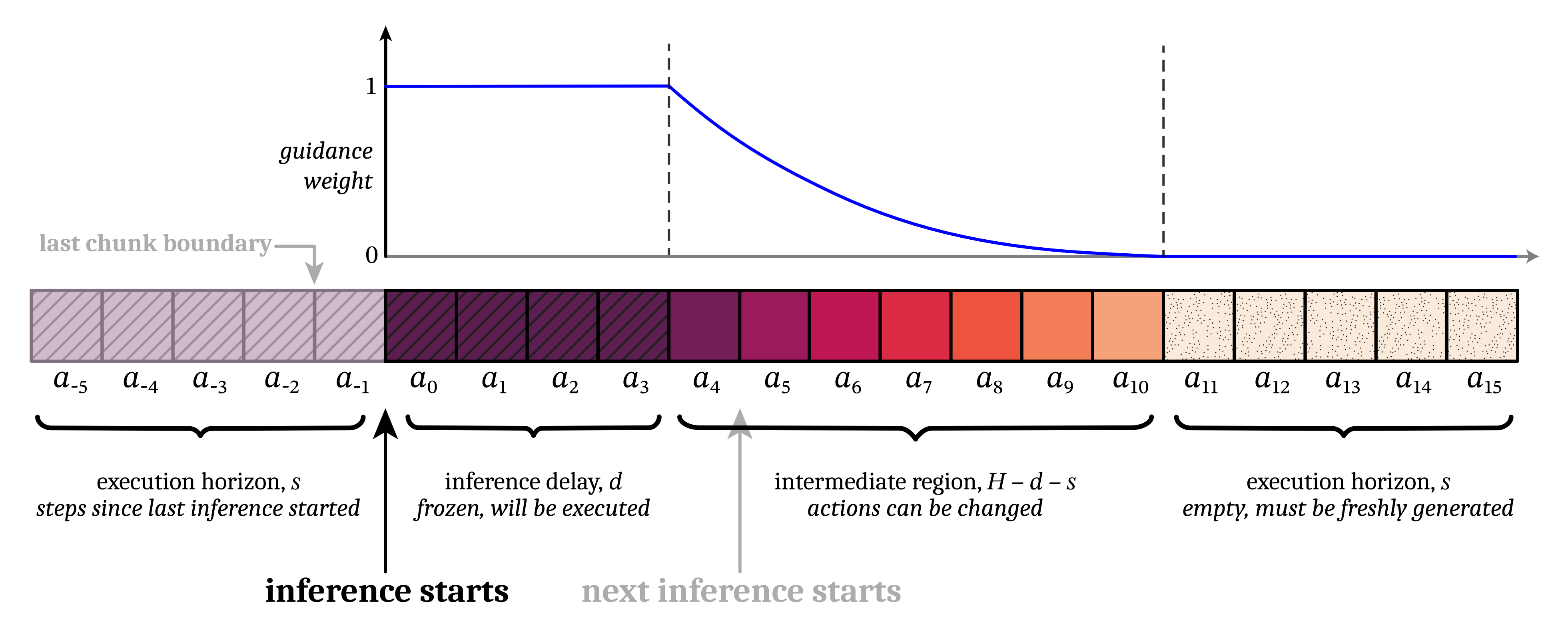

随后提出了 Train-time RTC https://hjfy.top/arxiv/2512.05964 。既然开始推理时刻需要基于上一个 chunk 的后缀进行 autograd inpainting，干脆直接在训练时让模型以上一个 chunk 的后缀（直接用 clean GT action）作为条件直接去噪，从而大幅节省 infer-time autograd 开销。由于不知道 infer-time 的真实 delay，训练时采用 randomly sampled delay.

Pi0.6 & Pi0.5 & Pi0 (6,7,8)

Pi0 除了以下设计，还引入了 zero-padding 进行跨本体混合训练，即状态和动作向量长度设定为数据集中最大自由度，不足补 0. 模型只能通过输入的本体感知 （例如 is_pad 信息？）和语言指令来识别当前的硬件构型. Pi0 并不能 zero-shot，但预训练能够帮助后训练的性能提升. 其他博主的一些理解：

Pi0 分离 actor 和 VLM，是为了避免后训练中对 VLM 能力的灾难性破坏.

Pi0 一次性引入了多个在后续被广泛使用的 Setting，当然，这些内容一开始的出处在这里不作考证，包括使用 MoT 进行 LLM 以及 Actor 的交互（见 Bagel ↗︎），使用 Flow Matching Loss 训练 Actor 以及使用 zero-padding 来进行跨本地的混合训练。

flowchart TD
    img["Images
(B, n_cam=3, H=224, W=224, C=3)"] --> siglip["PaliGemma Image Encoder(SigLIP)"]
    txt["Text Tokens
(B, max_token_len=48)"] --> tok["Gemma Token Embedding"]
    siglip --> vis["Visual Tokens
(B, 3*256=768, D=2048)"]
    tok --> textemb["Text Embeddings
(B, 48, D=2048)"]
    vis --> prefix["Prefix Tokens
(B, seq_len=816, D=2048)"]
    textemb --> prefix
    state["Robot State
(B, action_dim=32)"] --> stateproj["state_proj"]
    noisy["Noisy Actions x_t
(B, horizon=50, action_dim=32)"] --> actproj["action_in_proj"]
    time["Flow Time t
(B,)"] --> timemlp["Time Embedding MLP"]
    stateproj --> statetok["State Token
(B, 1, D=1024)"]
    actproj --> acttok["Action Tokens
(B, 50, D=1024)"]
    timemlp --> timetok["Time Tokens
(B, 50, D=1024)"]
    acttok --> mix["Action + Time Tokens
(B, 50, D=1024)"]
    timetok --> mix
    statetok --> suffix["Suffix Tokens
(B, seq_len=51, D=1024)"]
    mix --> suffix
    prefix --> pg["PaliGemma / Gemma 2B Expert"]
    suffix --> ae["Action Expert / Gemma 300M"]
    pg <--> shared["Shared Masked Self-Attn (qkv dim=256)"]
    ae <--> shared
    shared --> actout["action_out_proj"]
    actout --> vt["Predicted v_t
(B, 50, action_dim=32)"]
    gt["Target u_t = noise - action
(B, 50, action_dim=32)"] --> loss["Flow Matching Loss"]
    vt --> loss

其中一个 layer 的伪代码:

1
obs = norm_obs(obs0) # (B, Lo, 2048)
2
act = norm_act(act0) # (B, La, 1024)
3
q_obs = Wq_obs(obs).view(B, Lo, 8, 256).transpose(1, 2)   # (B, 8, Lo, 256)
4
k_obs = Wk_obs(obs).view(B, Lo, 1, 256).transpose(1, 2)   # (B, 1, Lo, 256)
5
v_obs = Wv_obs(obs).view(B, Lo, 1, 256).transpose(1, 2)   # (B, 1, Lo, 256)
6
q_act = Wq_act(act).view(B, La, 8, 256).transpose(1, 2)   # (B, 8, La, 256)
7
k_act = Wk_act(act).view(B, La, 1, 256).transpose(1, 2)   # (B, 1, La, 256)
8
v_act = Wv_act(act).view(B, La, 1, 256).transpose(1, 2)   # (B, 1, La, 256), Wv_act(act) is (B, La, 256)
9

10
q = cat([q_obs, q_act], dim=2)                            # (B, 8, Lo+La, 256)
11
k = repeat_kv(cat([k_obs, k_act], dim=2), n_rep=8)        # (B, 8, Lo+La, 256)
12
v = repeat_kv(cat([v_obs, v_act], dim=2), n_rep=8)        # (B, 8, Lo+La, 256)
13

14
y = softmax(q @ k.transpose(-2, -1)) @ v                  # (B, 8, Lo+La, 256)
15
y = y.transpose(1, 2).reshape(B, Lo+La, 2048)             # (B, Lo+La, 2048)
5 collapsed lines
16

17
obs_y = Wo_obs(y[:, :Lo])                                 # (B, Lo, 2048)
18
act_y = Wo_act(y[:, Lo:])                                 # (B, La, 1024)
19
obs1 = gated_residual(obs0, obs_y)                              # (B, Lo, 2048)
20
act1 = gated_residual(act0, act_y)                              # (B, La, 1024)

下面是 pi0.5. 一句话：对 state 进行 bin 离散并以文本丢进 VLM，预训练则对 action 使用 FAST[1] 分词器离散从而在不启用 action expert 的情况下进行 LLM-like NTP 预测并使用交叉熵 loss. 目的是大幅加快训练，而 infer-time 用 flow matching 反而更快。然而，对于跨本体 state 似乎没有做特殊处理，而都是归一化，可能需要通过语言指令来识别本体。

架构新技巧:

• pi0.5 flow time t 使用 adaRMSNorm[2] 用作 action flow condition. (pi0 是 MLP 直接为 token , concat action token)
• pi0.5 将 state 离散化为 task prompt（在 pi0 中，state 是过 linear 进 action expert）

1. FAST tokenizer 就是先将整个 action chunk (原文说了是 compressing the action chunks) 先 encode 为 8 个 latent 然后 vector quantize 就完事. 最终将 50x19 action 转为 8 个 token.
2. adarmsnorm:

   1
   # 1. 提取时间步 t 的正弦位置编码
   2
   # t: (b,)
   3
   # time_emb: (b, emb=2048)
   4
   time_emb = SinusoidalEmbedding(t, dim=2048)
   5
   # 2. 通过两层带 Swish 激活的 MLP 投影得到条件向量
   6
   # adarms_cond: (b, emb=2048)
   7
   adarms_cond = Swish(Linear(Swish(Linear(time_emb))))
   8
   # --- 以下发生在 Action Expert (Gemma-300m) 的每一层 Transformer Block 中 ---
   9
   # 3. 在 Action Expert 的每一层，将条件向量映射为缩放 (scale) 和平移 (shift) 参数
   10
   # scale, shift 形状均为 (b, emb=2048)
   11
   # 注意：由于 action_tokens 形状是 (b, ah=50, emb=2048)，这里会将 scale/shift 广播 (broadcast) 到序列长度维度
   12
   scale, shift = Linear(adarms_cond, out_features=2048 * 2).chunk(2, dim=-1)
   13
   # 4. 对隐藏层 x 应用 RMSNorm 后，注入时间信息
   14
   # x: (b, ah=50, emb=2048)
   15
   # x_out: (b, ah=50, emb=2048)
   1 collapsed line
   16
   x_out = RMSNorm(x) * (1 + scale.unsqueeze(1)) + shift.unsqueeze(1)

flowchart TD
    img["Images
(B, n_cam=3, H=224, W=224, C=3)"] --> siglip["PaliGemma Image Encoder(SigLIP)"]
    prompt["Task Prompt
(string)"] --> format["Prompt Format
Task: ..., State: ...;
Action:"]
    rawstate["Raw / Normalized Robot State
(B, action_dim=32)"] --> binstate["Digitize State
256 bins over [-1, 1]"]
    binstate --> statestr["State String
(e.g. '12 98 ...')"]
    statestr --> format
    format --> txt["Text + Discrete State Tokens
(B, max_token_len=200)"]
    txt --> tok["Gemma Token Embedding"]

    siglip --> vis["Visual Tokens
(B, 3*256=768, D=2048)"]
    tok --> textemb["Text/State Embeddings
(B, 200, D=2048)"]
    vis --> prefix["Prefix Tokens
(B, seq_len=968, D=2048)"]
    textemb --> prefix

    noisy["Noisy Actions x_t
(B, horizon=50, action_dim=32)"] --> actproj["action_in_proj"]
    time["Flow Time t
(B,)"] --> timemlp["Time MLP for adaRMSNorm"]

    actproj --> suffix["Suffix Action Tokens
(B, seq_len=50, D=1024)"]
    timemlp --> adarms["adaRMSNorm condition
(B, D=1024)"]

    prefix --> pg["PaliGemma / Gemma 2B Expert"]
    suffix --> ae["Action Expert / Gemma 300M"]
    adarms --> ae

    pg <--> shared["Shared Masked Self-Attn
(qkv head_dim=256)"]
    ae <--> shared

    shared --> actout["action_out_proj"]
    actout --> vt["Predicted v_t
(B, 50, action_dim=32)"]
    gt["Target u_t = noise - action
(B, 50, action_dim=32)"] --> loss["Flow Matching Loss"]
    vt --> loss

pi0.6

flowchart TD
    img["Images
(B, n_cam=3, H=224, W=224, C=3)"] --> siglip["Image Encoder
SigLIP 400M"]
    txt["Text + Discrete State Tokens
(B, max_token_len=200)"] --> tok["Gemma Token Embedding"]

    siglip --> vis["Visual Tokens
(B, n_cam*256, D_vlm)"]
    tok --> textemb["Text/State Embeddings
(B, 200, D_vlm)"]
    vis --> prefix["Prefix Tokens
(image + text + state + metadata)"]
    textemb --> prefix

    noisy["Noisy Actions a_eta
(B, horizon=50, action_dim=32)"] --> actproj["action_in_proj"]
    time["Flow Time eta
(B,)"] --> timemlp["Time MLP for adaRMSNorm"]

    actproj --> suffix["Suffix Action Tokens
(B, seq_len=50, D_ae)"]
    timemlp --> adarms["adaRMSNorm condition
(B, D_ae)"]

    prefix --> pg["pi*0.6 VLA Backbone
Gemma 3 4B"]
    suffix --> ae["Action Expert
860M"]
    adarms --> ae

    pg <--> shared["Shared Masked Self-Attn
(qkv head_dim=256)"]
    ae <--> shared

    shared --> actout["action_out_proj"]
    actout --> vt["Predicted Flow f_theta
(B, 50, action_dim=32)"]
    gt["GT Action Chunk a
(B, 50, action_dim=32)"] --> ftarget["Target omega - a
(B, 50, action_dim=32)"]
    noise["Noise omega ~ N(0,I)
(B, 50, action_dim=32)"] --> noisy
    noise --> ftarget
    ftarget --> floss["Flow Matching Loss
alpha_eta * ||f_theta - (omega - a)||^2"]
    vt --> floss

    img --> vfsiglip["Value Image Encoder
SigLIP 400M"]
    txt --> vftok["Value Text Embedding"]
    vfsiglip --> vfprefix["Value Prefix Tokens"]
    vftok --> vfprefix
    vfprefix --> vf["Value Function
Gemma 270M + value head"]
    vf --> vdist["Value Distribution
p_phi(V | o_t, l), 201 bins"]
    returns["MC Return R_t
from success/failure episode reward"] --> vloss["Value CE Loss
CE(p_phi, discretized R_t)"]
    vdist --> vloss
    vdist --> vscalar["Scalar Value V(o)
E over value bins"]
    vscalar --> adv["Advantage A(o,a)
r_t:t+N + V(o_t+N) - V(o_t)"]
    adv --> bin["Binarize
I_t = 1[A > epsilon_l]"]
    bin --> advtxt["Advantage Text Token
'positive' / 'negative'"]
    advtxt --> tok

    pg --> subtask["Subtask Text Tokens
(e.g. 'tamp the coffee')"]
    pg --> fastout["FAST Discrete Action Tokens
a^l_t:t+H"]
    gt --> fasttok["FAST Tokenizer"]
    fasttok --> fastgt["GT FAST Action Tokens"]
    subtask --> tokce["Next-token CE/NLL
subtask + FAST action tokens"]
    fastout --> tokce
    fastgt --> tokce

    classDef pi06 fill:#fff2b3,stroke:#d6a600,stroke-width:2px,color:#111;
    class pg,ae,vfsiglip,vftok,vfprefix,vf,vdist,vscalar,adv,bin,advtxt,fastout,fasttok,fastgt,tokce pi06;

总结

VLA 架构的大方向:

1. [VLM] -> embedding -> [MLP(i.e. action head)] -> action
2. [VLM] -> embedding -> kv -> [Decoder transformer, attended by learnable q pos embedding] -> [action head] -> action (ACT-like)
3. [VLM] -> MoT <-> [action expert] -> [action head] -> action (Pi-like)