285-hw2: Policy Gradients

回忆提纲

实现 PG, baseline-PG(actor-critic) 和 GAE.

Takeaways:

训练更稳定的方法
1. large batch (10000 vs 1000),
2. reward-to-to(gamma=0.95 衰减 vs 每一步优势函数=整条轨迹G),
3. normalized advantage，直接整个 batch advantages = (advantages - mean) / (std + 1e-8)
4. critic gradient steps: 每次拿到 obs 和 q_values 执行多次 critic.update()
5. GAE (lambda = 0.95 ~ 0.99)

Experiment 1 (CartPole, REINFORCE):

回答问题

大 batch vs 小 batch（忘记截图 eval 了，never mind）:

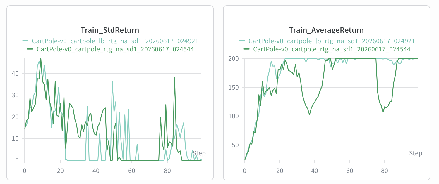
在大 batch 情况下，是否开启 na 和 reward-to-go

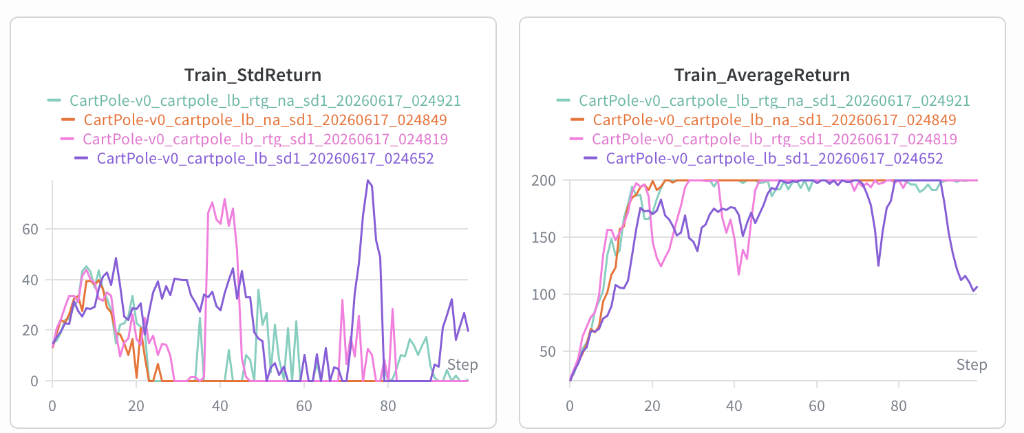
Which value estimator has better performance without advantage normalization: the trajectory- centric one, or the one using reward-to-go?

rtg.

Between the two value estimators, why do you think one is generally preferred over the other?

rtg. 因为这样能反映每个 action 的 value 而不是整条轨迹，更好学习. [ai]: 减少 credit assignment 的噪声 i.e. 减少“把奖励归因给不相关动作”的情况.

Did advantage normalization help?

yes.

Did the batch size make an impact?

yes.

exact command:

[email protected]
/hw285.git ; cd hw2
uv run src/scripts/run.py —env_name CartPole-v0 -n 100 -b 1000
-exp_name cartpole # 直接使用了 pdf 的命令

解题过程失误

get_action 不是 argmax 使用最大概率的策略而应当使用 dist=torch.distributions.Categorical(logits=logits) 然后 dist.sample(). 那种 argmax 写法是 LLM 的.
求梯度不是 -prob * advantage 别忘了是 -log_prob * advantages
除以 std 需要 std + 1e-8

回忆提纲

思路：

是 REINFORCE（或者 vanilla Policy Gradient）方法。policy 输入 obs 输出离散 action_prob。(monte-carlo) 用当前 policy 概率 sample discrete action 然后 rollout 多条轨迹得到一个 batch，直接计算总奖励（称为 advantages，可选开启 reward-to-go 即 Σ(γ^t r_t)）后交给 policy 用 loss = -log_prob * advantages 直接更新即可.

代码技巧：

代码中每次 forward 的实际 batch size 确实是不一样的。因为代码 rollout 过程是采样一整条 traj，traj 的每个 action step 作为一个 sample，所以 batch 可能是 20 + 17 + ... 这样随机累加直到满足预定 batch size.
默认 MLP: 2 隐藏层，每层 64 神经元. 本任务输入是 4 维观测 [小车位置, 小车速度, 杆子角度, 杆尖角速度]，输出是 1 个离散动作（2 选 1：向左或向右推小车）

Experiment 2 (HalfCheetah, Monte-Carlo + Baseline，Actor-Critic)

回答问题

no baseline | baseline | baseline + na | baseline + smaller baseline gradient step（都开 rtg）: https://wandb.ai/julyfun-collect-shanghai-jiao-tong-university/cs285_hw2/workspace?nw=nwuserjulyfuncollect

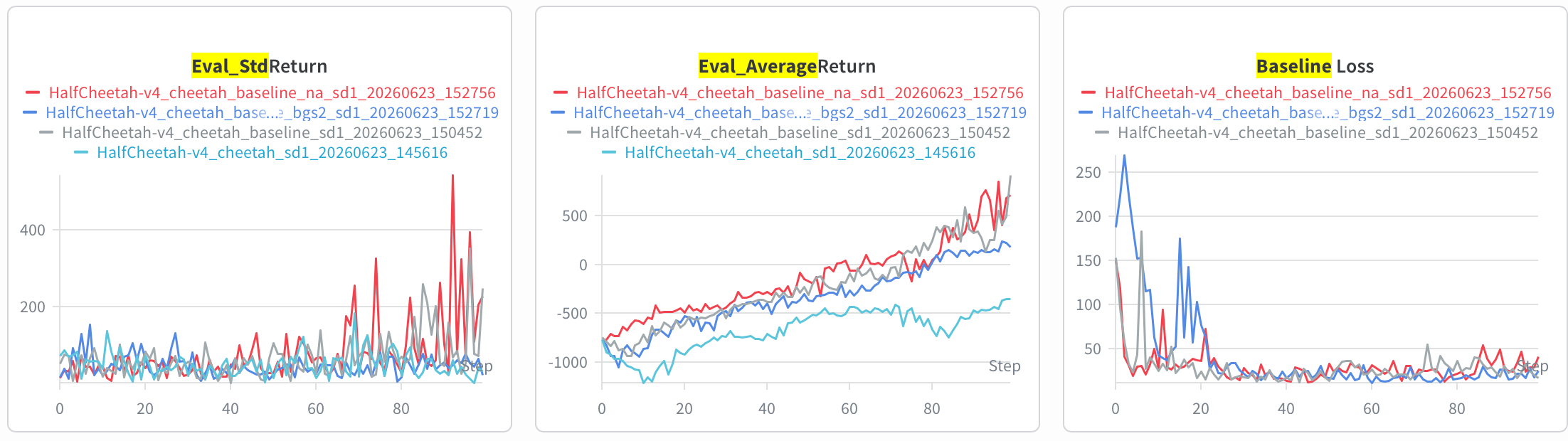
bgs 的作用？

bgs 小了以后，baseline loss 下降更慢，return 上升更慢.

na 的效果？

no-baseline + na 也取得了不错的效果，说明 na 确实很强大。当然 baseline + na 上升似乎更快，但是最后 StdReturn 很不稳定了，不知道咋回事.

exact command:

uv run src/scripts/run.py --env_name HalfCheetah-v4 -n 100 -b 5000 -eb 3000 -rtg \ --discount 0.95 -lr 0.01 --use_baseline -blr 0.01 --exp_name cheetah_baseline_bgs2 -bgs 2

解题过程失误

get_action 又写错了，应该是用 mean + sample(logstd) 采样，我一开始写成了直接 return mean
update() 不用手算概率密度，直接 dist.log_prob() 就行.
起初的 avg return 很低，长期 -700。我还以为写挂了，跑到 50 轮以上才显著为正。

回忆提纲

思路：

这其实就是 Actor-Critic。在 REINFORCE 基础上，开一个 value_net，然后 advantages = monte_carlo_q_values - value_net(obs). 每个 iteration 先更新 policy 后更新 value_net. 而 value_net 的更新就是 F.mse_loss(self.forward(obs), monte_carlo_q_values)
从这个实验开始支持连续动作。对于连续动作使用了 mean_net 网络配合 logstd 参数，计算概率改为计算概率密度（直接用 torch.distributions.Normal(mean, self.logstd.exp())）

技巧:

这部分并不是 Time-delta，而是 Σ(γ^t r_t) - V(s)，下一章才开始用 time-delta（默认是单步的，形式为 r + γ*V(s+1) - V(s))

Experiment 3: GAE

回答问题

• Submit the logs of the five experiments above with λ ∈{0,0.95,0.98,0.99,1}. The best run should achieve an average return above 150 at least once during training. Results may have some variance and you might need to give it another try to get a good run.

好的.

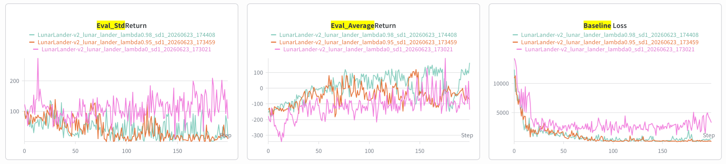
• Provide a single plot with the learning curves for the LunarLander-v2 experiments that you tried. Describe in words how λ affected task performance.

λ=0 时是单步 TD，return 方差大上升不稳定，baseline 很难学会。 λ=1 时方差也比较大，但 return 还可以。λ=0.98/0.99 最好.

1.0 vs 0.99 vs 0.98:

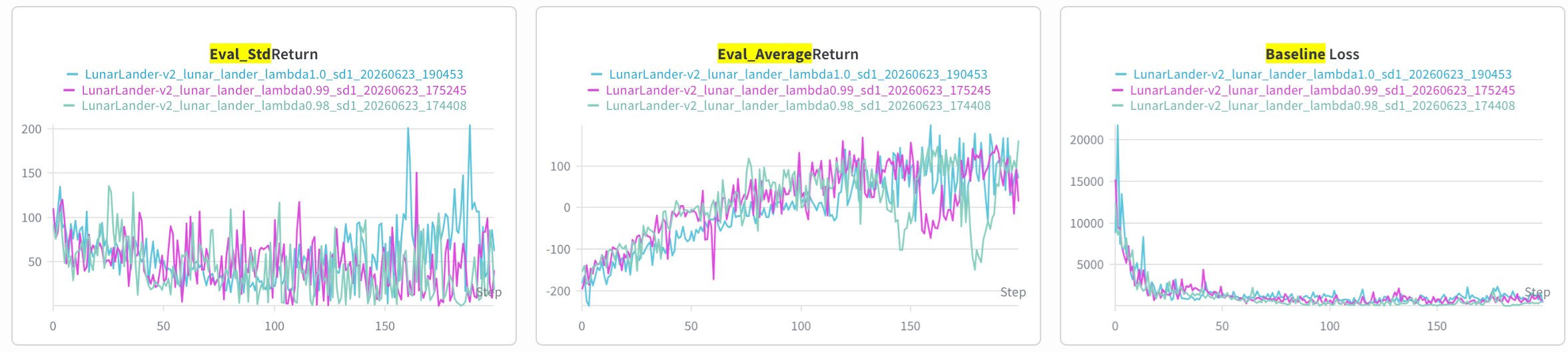
0.98 vs 0.95 vs 0:

火箭软着陆动图：https://wandb.ai/julyfun-collect-shanghai-jiao-tong-university/cs285_hw2/runs/0xalwgv3?nw=nwuserjulyfuncollect

• Consider the parameter λ. What does λ= 0 correspond to? What about λ= 1? Relate this to the task performance in LunarLander-v2 in one or two sentences.

1
for i in reversed(range(batch_size)): # 没错 batch 中的每一个 sample 是一个连续的 rollout step
2
    advantages[i] = rewards[i] + (1.0 - terminals[i]) * self.gamma * values[i + 1] - values[i] \
3
        + self.gamma * self.gae_lambda * advantages[i + 1]

从上述代码看出，λ=0 就是使用单步 TD 优势函数 (在作业中即符号 )，具有尚未学成的神经网络导致的 high bias 和去除 monte-carlo 带来的 low variance. λ = 1 则所有 time-delta 权重一样，是一种四不像方法，high variance.

• Provide the exact command line configurations you used to run your experiments, including any param- eters changed from defaults

1
for i in 0 0.95 0.98 0.99 1.0
2
    uv run src/scripts/run.py --env_name LunarLander-v2 --ep_len 1000 --discount 0.99 \
3
        -n 200 -b 2000 -eb 2000 -l 3 -s 128 -lr 0.001 --use_reward_to_go --use_baseline \
4
        --gae_lambda $i --exp_name lunar_lander_lambda$i --video_log_freq 10
5
end

回忆提纲

思路：

GAE 就是先 monte-carlo 然后对每一步都求 TD r + γ*V(s+1) - V(s)，然后给这些 TD 分配 λ 衰减的权重.
相比上一章只加了 GAE，它就是一个循环。

Experiment 4: Hyperparameter

• Submit the log of the run with the best performance. The best run should reach an average return of 1000 at least once within 100K environment steps. Again, results may vary with different random seeds. (Note: For this reason, in actual RL research, it is generally very important to report results averaged over multiple random seeds to ensure statistical significance and avoid cherry-picking! However, for this assignment, we only require you to submit your best run to reduce computational burden.)

• Provide the best set of hyperparameters on InvertedPendulum-v4 and the exact command line config- uration. Briefly discuss which hyperparameters mattered in your tuning process.

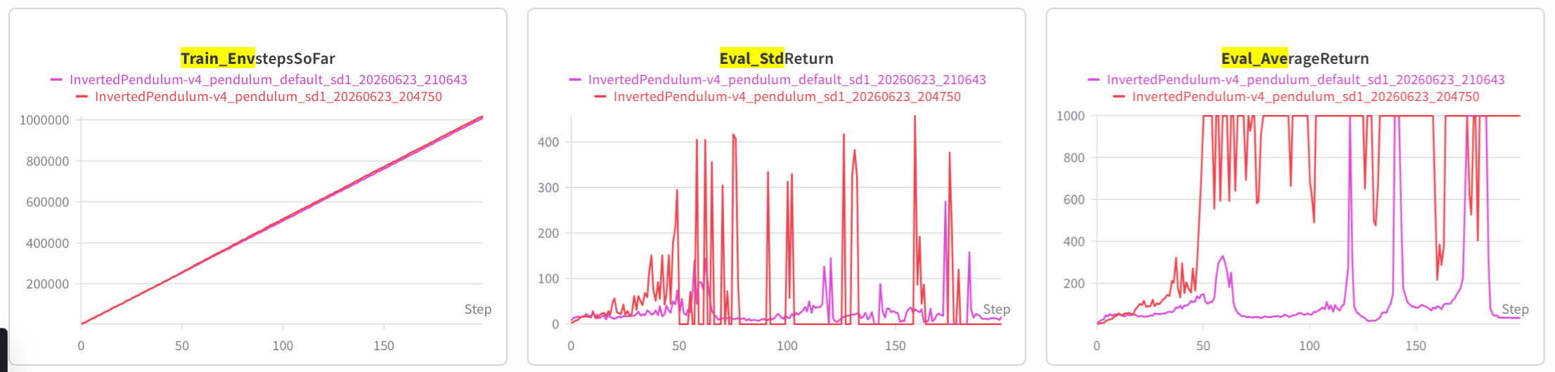
1
uv run src/scripts/run.py --env_name InvertedPendulum-v4 -n 200 -b 5000 -eb 1000 --use_reward_to_go --use_baseline --normalize_advantages --gae_lambda 0.99 --discount 0.95 \
2
    --exp_name pendulum --video_log_freq 10

该命令产生了下图中的红色曲线。而紫色曲线则是 pdf 中的默认命令（n_iter 改成 200，总共约 100K steps.）

• Show learning curves for the average returns with your hyperparameters and with the default settings, with environment steps on the x-axis.

x 轴我就不换了。

其他实验

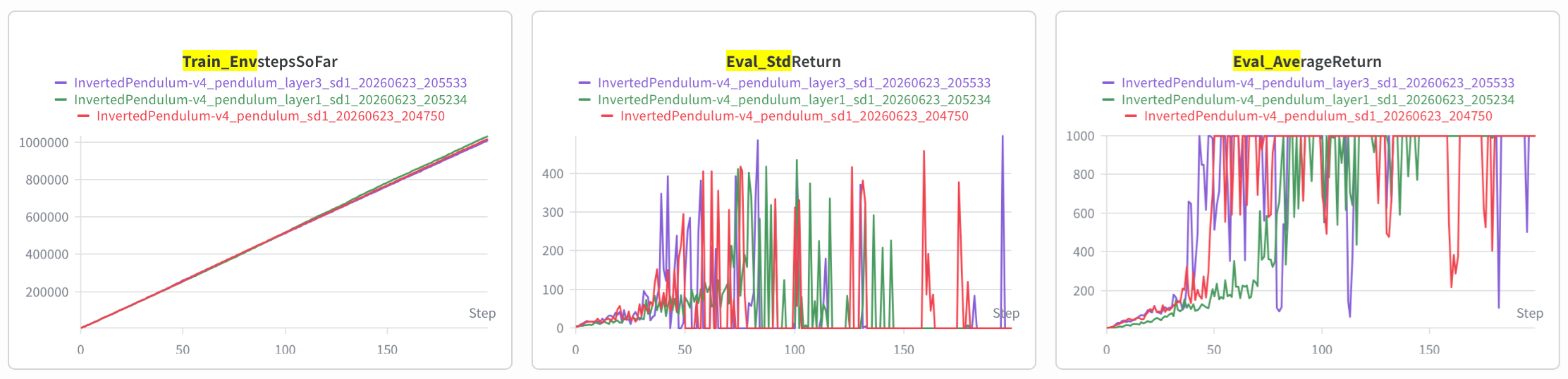
n_layer 1 vs 2 vs 3 （红色为默认的 2）:

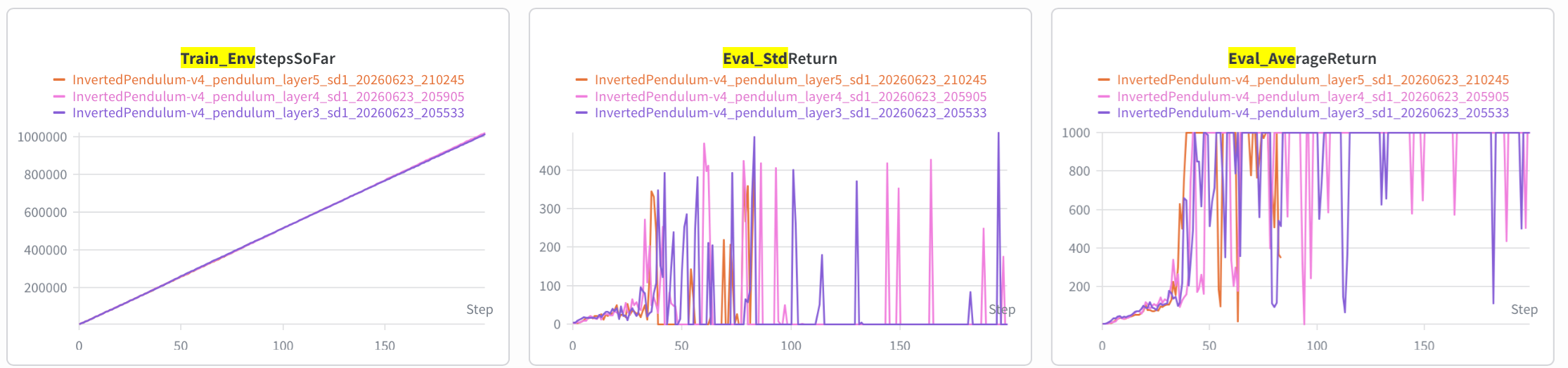
n_layer 3 vs 4 vs 5，可以看出来差不多：

回忆提纲

InvertedPendulum-v4 任务输入输出维度以及含义？1句话

GPT5.5 InvertedPendulum-v4 的输入观测是 4 维，通常表示小车位置、小车速度、杆角度相关量和杆角速度；输出动作是 1 维连续力，表示施加在小车上的水平推力。