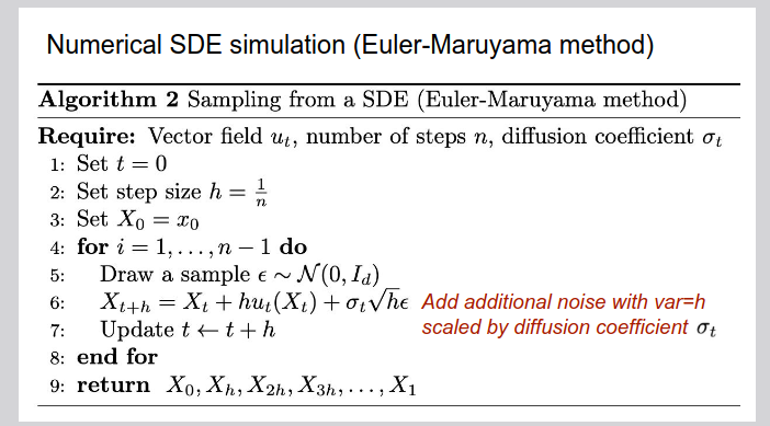
- ODE(常微分方程) SDE(随机微分方程, 带随机波动的变化)
- SDE: 系统的未来状态不仅依赖当前状态,还包含非决定性的随机波动(噪声),因此未来状态是一个概率分布. 方程中多了随机项(通常用布朗运动表示)
- CFM: ?
- 教材笔记,详实简单: https://arxiv.org/pdf/2506.02070
- Lab: https://github.com/eje24/iap-diffusion-labs
Lec 1
- https://diffusion.csail.mit.edu/docs/slides_lecture_1.pdf
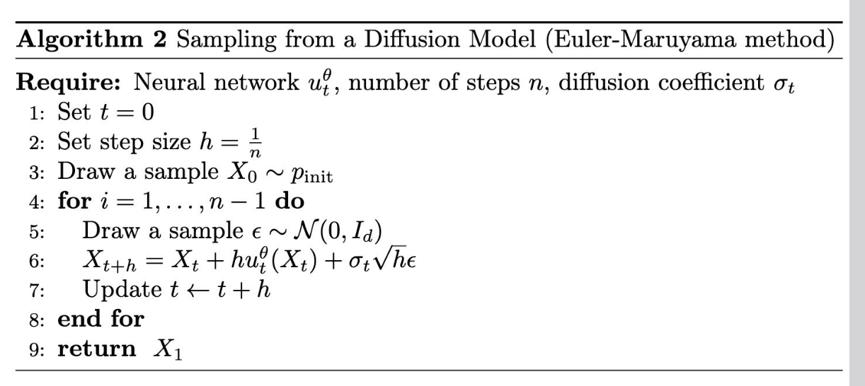
- Diffusion network 预测的就是向量场(输入: t, X 当前位置. 输出: X 速度)

- 改为神经网络形式(引入 $theta$). 注意这里 $sigma_t$ 可以由时间变化:
- [qm] 为何噪声到图像的过程可以建模为带布朗运动的 SDE?
Lec 2
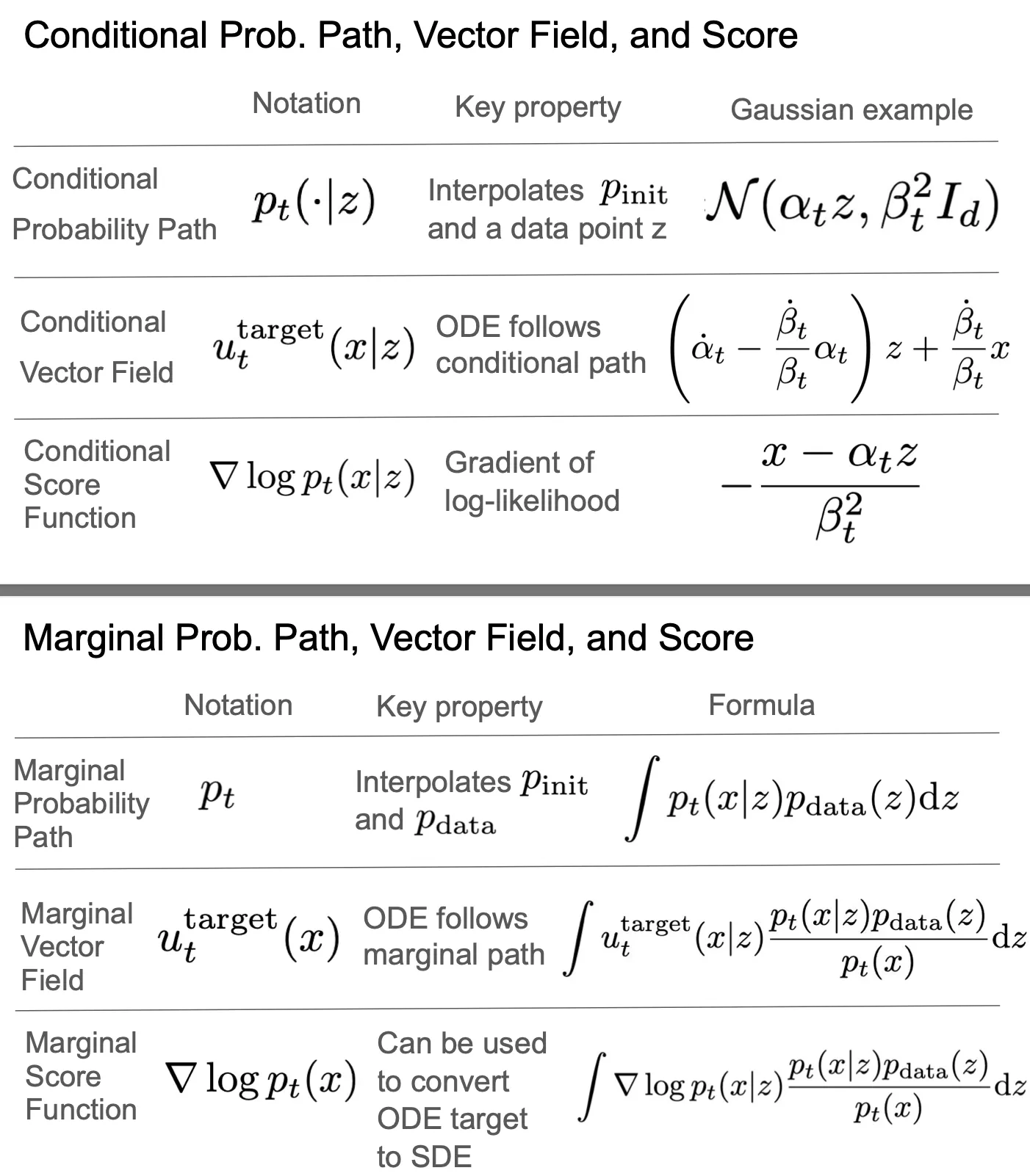
- Conditional Probability Path: 给定目标点 $z$(例如 diffusion 中的最终图像),求 $x$ 下一步路径
- Marginal Probability Path: 不给定条件(所有分布的加权平均),求下一步路径
- 两者在 $t_0$ 是完全一样的,从第二步开始才有区别.
- 向量场函数(也可视为梯度或者速度):$$“def” u(x: RR^d, t: [0, 1]) |-> RR^d$$
- [qm] 为何 score function 这样定义
[附]
Lec3 ok
Lec4: Guided (conditional) DDM
- https://github.com/eje24/iap-diffusion-labs/blob/main/solutions/lab_three_complete.ipynb
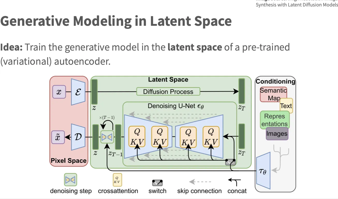
- condition 是怎么加入 UNet: 自己看代码无需多言.
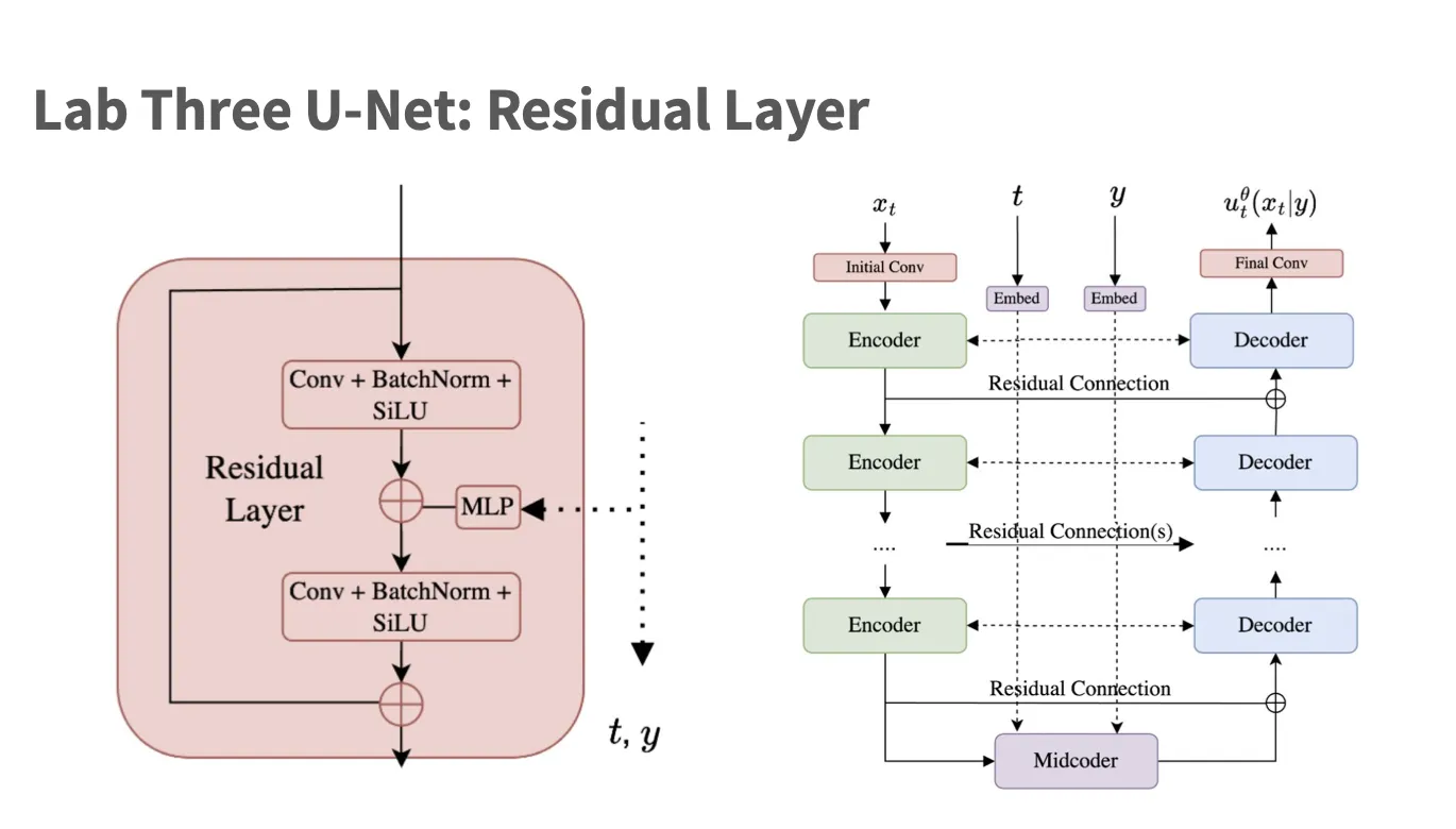
1class ResidualLayer(nn.Module):2 def __init__(self, channels: int, time_embed_dim: int, y_embed_dim: int):3 super().__init__()4 self.block1 = nn.Sequential(5 nn.SiLU(),6 nn.BatchNorm2d(channels),7 nn.Conv2d(channels, channels, kernel_size=3, padding=1)8 )9 self.block2 = nn.Sequential(10 nn.SiLU(),11 nn.BatchNorm2d(channels),12 nn.Conv2d(channels, channels, kernel_size=3, padding=1)13 )14 # Converts (bs, time_embed_dim) -> (bs, channels)15 self.time_adapter = nn.Sequential(36 collapsed lines
16 nn.Linear(time_embed_dim, time_embed_dim),17 nn.SiLU(),18 nn.Linear(time_embed_dim, channels)19 )20 # Converts (bs, y_embed_dim) -> (bs, channels)21 self.y_adapter = nn.Sequential(22 nn.Linear(y_embed_dim, y_embed_dim),23 nn.SiLU(),24 nn.Linear(y_embed_dim, channels)25 )26
27 def forward(self, x: torch.Tensor, t_embed: torch.Tensor, y_embed: torch.Tensor) -> torch.Tensor:28 """29 Args:30 - x: (bs, c, h, w)31 - t_embed: (bs, t_embed_dim)32 - y_embed: (bs, y_embed_dim)33 """34 res = x.clone() # (bs, c, h, w)35
36 # Initial conv block37 x = self.block1(x) # (bs, c, h, w)38
39 # Add time embedding40 t_embed = self.time_adapter(t_embed).unsqueeze(-1).unsqueeze(-1) # (bs, c, 1, 1)41 x = x + t_embed42
43 # Add y embedding (conditional embedding)44 y_embed = self.y_adapter(y_embed).unsqueeze(-1).unsqueeze(-1) # (bs, c, 1, 1)45 x = x + y_embed46
47 # Second conv block48 x = self.block2(x) # (bs, c, h, w)49
50 # Add back residual51 x = x + res # (bs, c, h, w)不禁令人发现:
- 自然语言适合描述低频信号,而不擅长描述高频信号
- UNet 通过保留高频信号来抑制信息过于平滑的问题
- 之所以“视频能展示的内容远少于占用空间相同的游戏”是因为 mp4 需要编码高频信号
- AE 压缩为低维潜在向量的结构之所以能用于生成,是因为它强制学习数据的底层结构
Some question
- 这里如何编码时间 (bs, 1, 1, 1) => (bs, emb_dim)?用了 nn.Parameter.
- 可能也可以用无需学习的正弦余弦位置编码
1class FourierEncoder(nn.Module):2 """3 Based on https://github.com/lucidrains/denoising-diffusion-pytorch/blob/main/denoising_diffusion_pytorch/karras_unet.py#L1834 """5 def __init__(self, dim: int):6 super().__init__()7 assert dim % 2 == 08 self.half_dim = dim // 29 self.weights = nn.Parameter(torch.randn(1, self.half_dim))10
11 def forward(self, t: torch.Tensor) -> torch.Tensor:12 """13 Args:14 - t: (bs, 1, 1, 1)15 Returns:7 collapsed lines
16 - embeddings: (bs, dim)17 """18 t = t.view(-1, 1) # (bs, 1)19 freqs = t * self.weights * 2 * math.pi # (bs, half_dim)20 sin_embed = torch.sin(freqs) # (bs, half_dim)21 cos_embed = torch.cos(freqs) # (bs, half_dim)22 return torch.cat([sin_embed, cos_embed], dim=-1) * math.sqrt(2) # (bs, dim)